ClearMap Image Analysis Tools

Here we introduce the main image processing steps for the detection of nuclear-located signal with examples.

The data is a small region isolated from an iDISCO+ cleared mouse brain immunostained against c-fos. This small stack is included in the ClearMap package in the Test/Data/ImageAnalysis/ folder:

>>> import os
>>> import ClearMap.IO as io
>>> import ClearMap.Settings as settings
>>> filename = os.path.join(settings.ClearMapPath, \
>>>                         'Test/Data/ImageAnalysis/cfos-substack.tif');

Visualizing 3D Images

Large images in 3d are best viewed in specialized software, such as Imaris for 3D rendering or ImageJ to parse the stacks. For the full size data, it is recommended to open the stacks in ImageJ using the « virtual stack » mode.

In ClearMap we provide some basic visualization tools to inspect the 3d data in the module ClearMap.Visualization.Plot.

To load them run

>>> import ClearMap.Visualization.Plot as plt

Tiled Plots

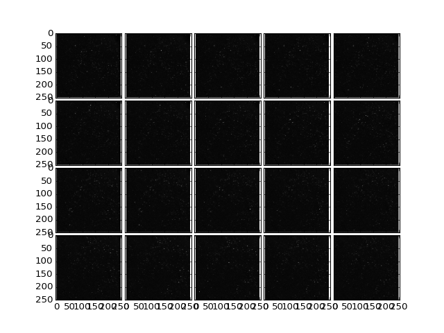
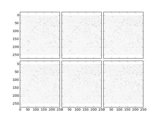
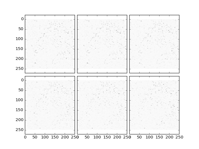
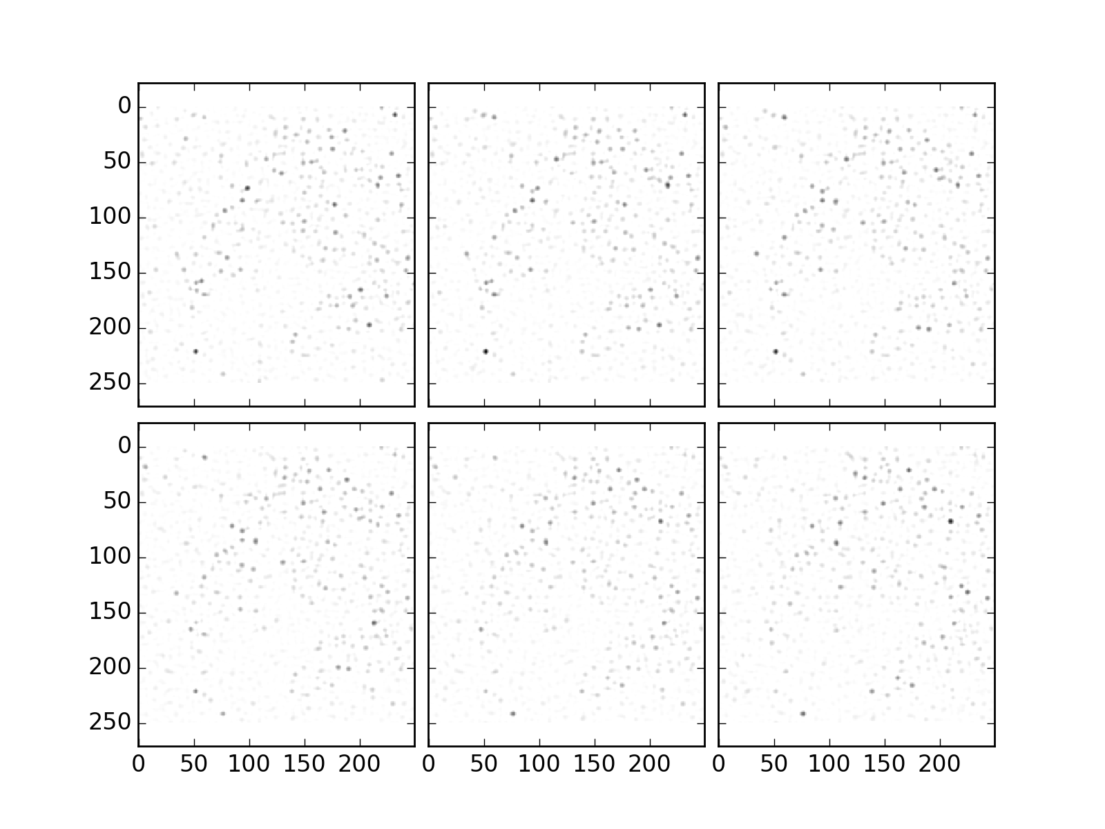
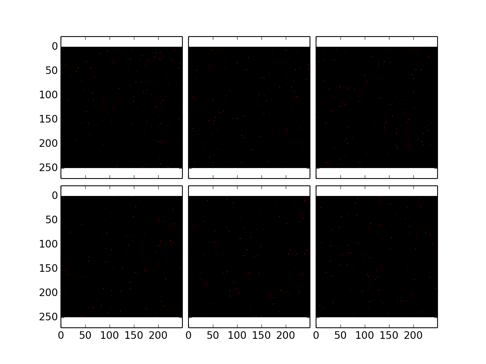
In our experience results of 3d image analysis is inspected most accurately by plotting each horizontal plane in the image in tiles that are coupled for zooming. Intermediate results from all the steps of the SpotDetection can also be written as image stacks and opened with ImageJ.

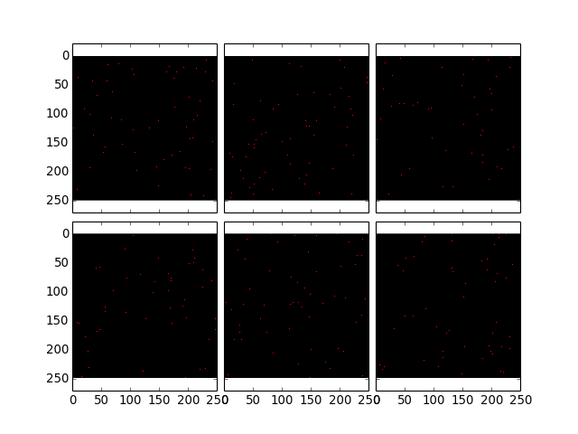
>>> data = io.readData(filename, z = (0,26));
>>> plt.plotTiling(data);

(Source code, png, hires.png, pdf)

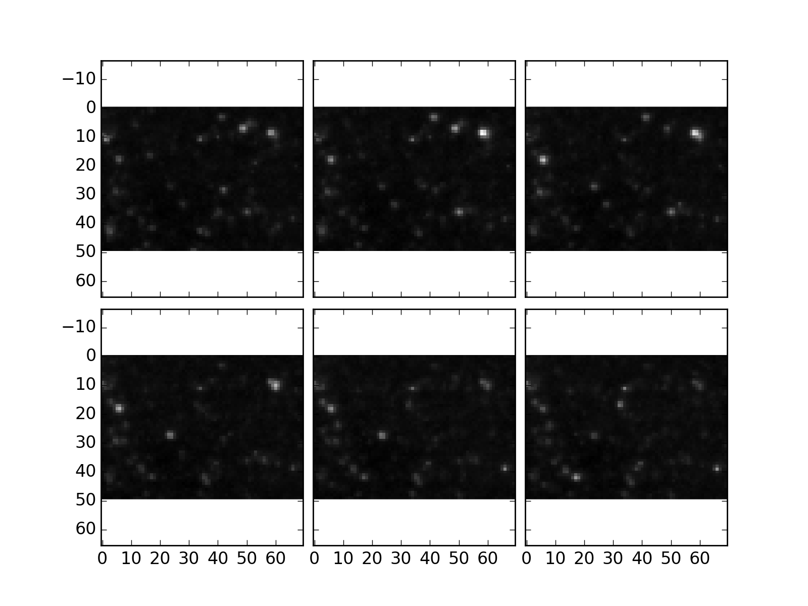
To only plot a particular subregion its possible to specify the x,y,z range.

>>> plt.plotTiling(data, x = (0,70), y = (0,50), z = (10,16));

(Source code, png, hires.png, pdf)

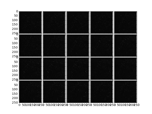
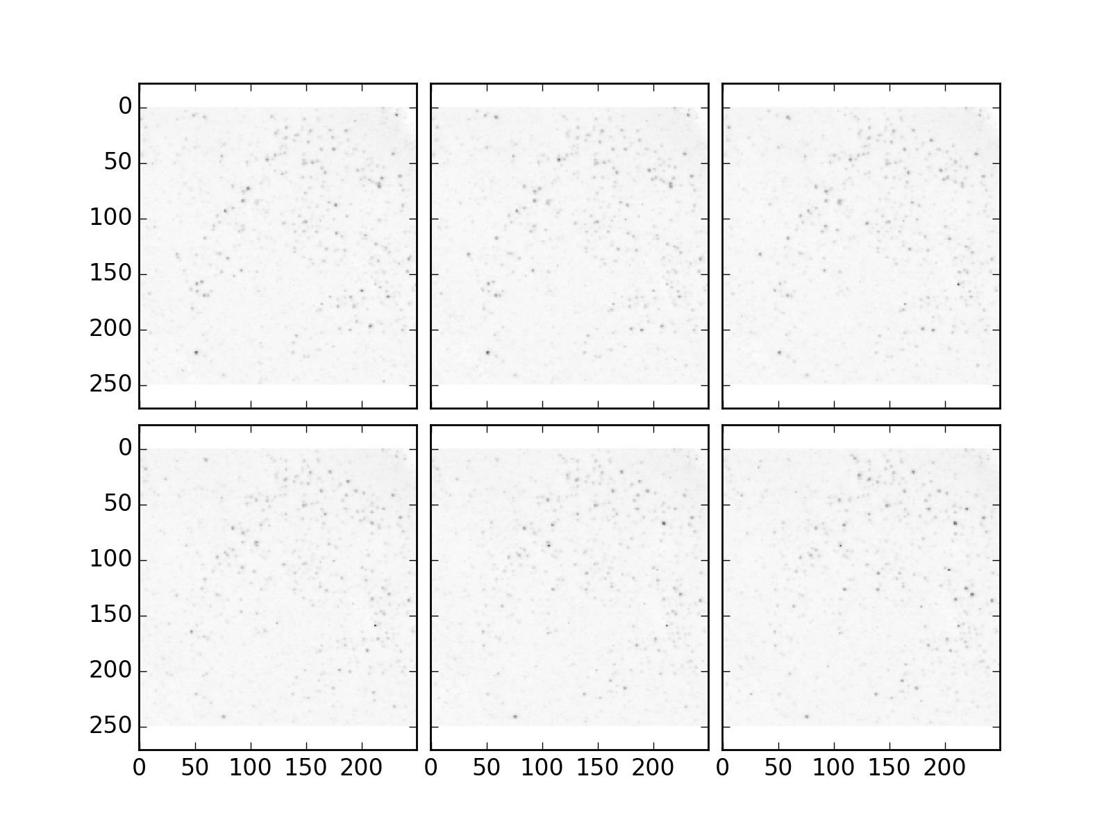
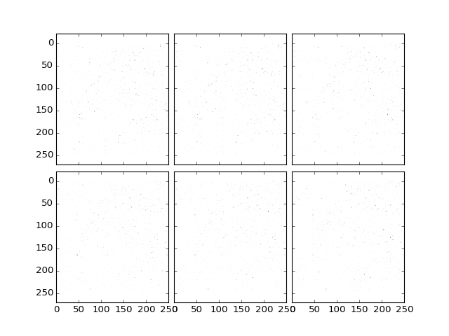
Sometimes inverse colors may be better:

>>> plt.plotTiling(data, inverse = True,  z = (10,16));

(Source code, png, hires.png, pdf)

Image Statistics

It is useful to gather some information about the image initially. For larger images that don’t fit in memory in ClearMap certain statistics can be gathered in parallel via the module ClearMap.ImageProcessing.ImageStatistics module.

>>> import ClearMap.ImageProcessing.ImageStatistics as stat
>>> print stat.calculateStatistics(filename, method = 'mean')
2305.4042155294119

To get more information about the progress use the verbose option

>>> print stat.calculateStatistics(filename, method = 'mean', verbose = True)
ChunkSize: Estimated chunk size 51 in 1 chunks!
Number of SubStacks: 1
Process 0: processing substack 0/1
Process 0: file          = /ClearMap/Test/Data/ImageAnalysis/cfos-substack.tif
Process 0: segmentation  = <function calculateStatisticsOnStack at 0x7fee9c25dd70>
Process 0: ranges: x,y,z = <built-in function all>,<built-in function all>,(0, 51)
Process 0: Reading data of size (250, 250, 51): elapsed time: 0:00:00
Process 0: Processing substack of size (250, 250, 51): elapsed time: 0:00:00
Total Time Image Statistics: elapsed time: 0:00:00
2305.4042155294119

Image statistics can be very helpful for modules, such as Ilastik, requiring a different bit depth than the original 16 or 12 bits files, as it helps to determine how to resample the images to a lower bit depth.

Background Removal

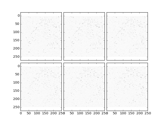
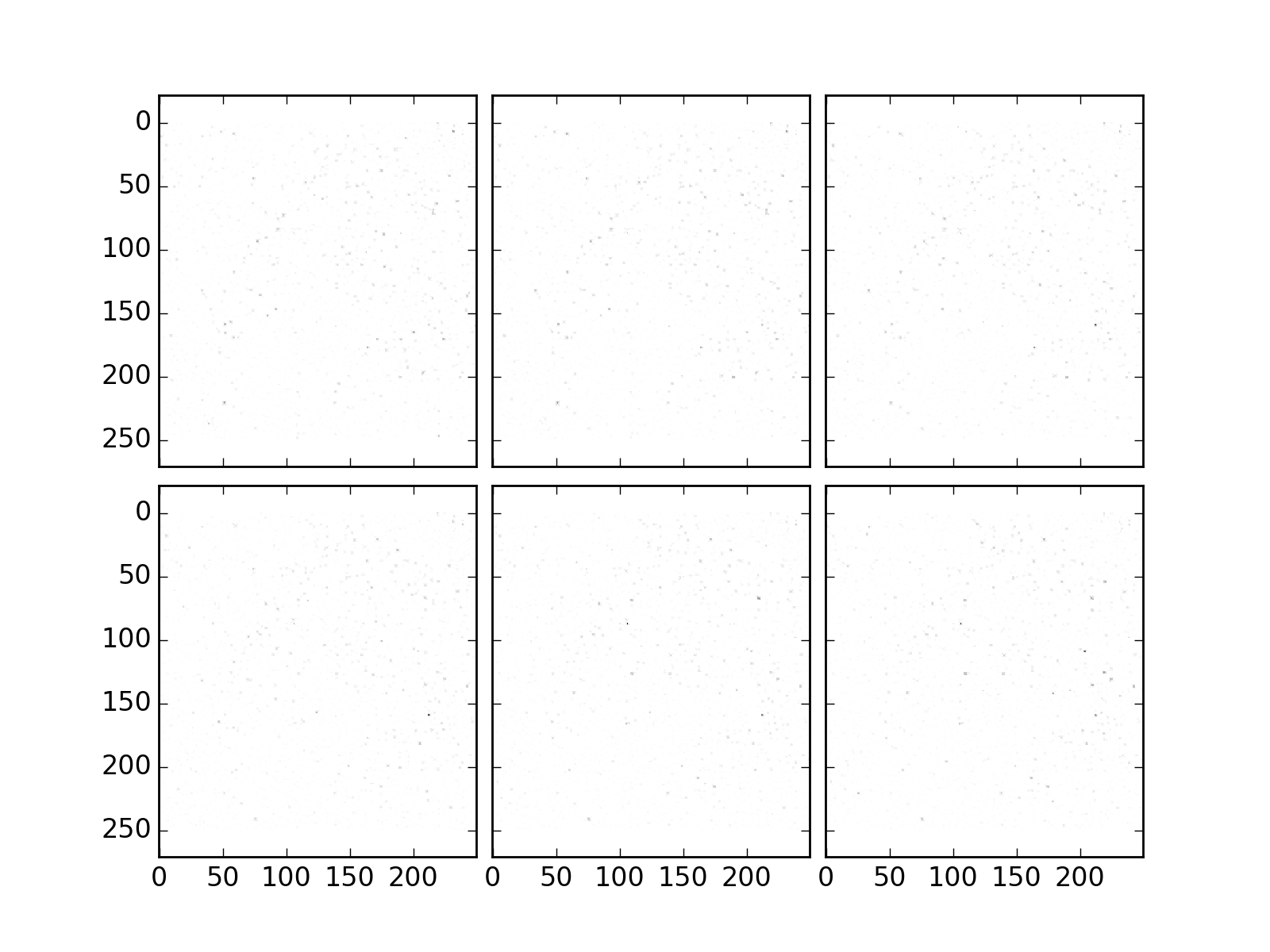
One of the first steps is often to remove background variations. The ClearMap.Imageprocessing.BackgroundRemoval module can be used. It performs the background subtraction by morphological opening. The parameter is set as (x,y) where x and y are the diameter of an ellipsoid of a size close to the typical object detected in pixels. The intensity of the signal is greatly reduced after the filtering, but the signal-to-noise ration is increased:

>>> import ClearMap.ImageProcessing.BackgroundRemoval as bgr
>>> dataBGR = bgr.removeBackground(data.asype('float'), size=(5,5), verbose = True);
>>> plt.plotTiling(dataBGR, inverse = True, z = (10,16));

(Source code, png, hires.png, pdf)

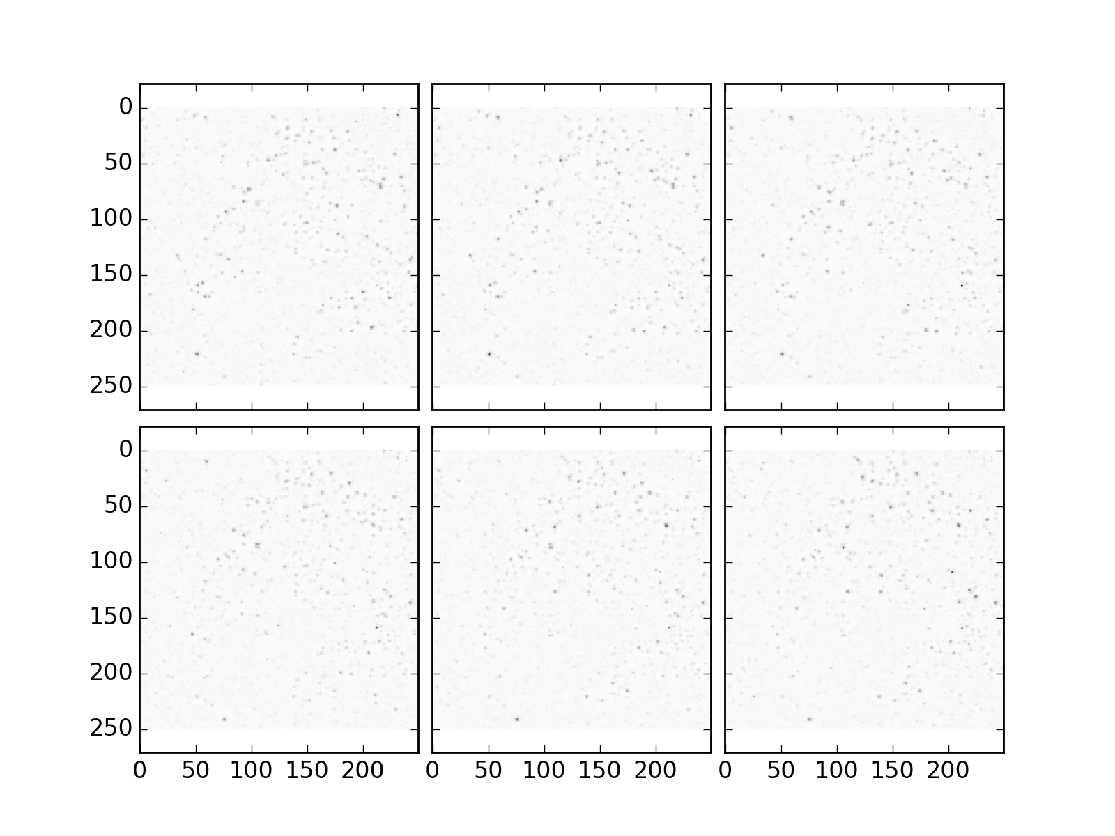
Note that if the background feature size is chosen too small, this may result in removal of cells:

>>> dataBGR = bgr.removeBackground(data.astype('float'), size=(3,3), verbose = True);
>>> plt.plotTiling(dataBGR, inverse = True, z = (10,16));

(Source code, png, hires.png, pdf)

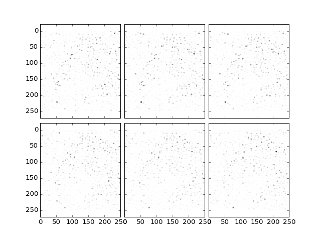
Image Filter

A useful feature is to filter an image. Here the ClearMap.Imageprocessing.Filter package can be used.

To detect cells center, the difference of Gaussians filter is a powerful way to increase the contrast between the cells and the background. The size is set as (x,y,z), and usually x, y and z are about the typical size in pixels of the detected object. As after the background subtraction, the intensity of the signal is again reduced after the filtering, but the signal-to-noise ration is dramatically increased:

>>> from ClearMap.ImageProcessing.Filter.DoGFilter import filterDoG
>>> dataDoG = filterDoG(dataBGR, size=(8,8,4), verbose = True);
>>> plt.plotTiling(dataDoG, inverse = True, z = (10,16));

(Source code, png, hires.png, pdf)

Maxima Detection

The ClearMap.ImageProcessing.MaximaDetection module contains a set of useful functions for the detection of local maxima. A labeled image can be visualized using the ClearMap.Visualization.Plot.plotOverlayLabel() routine.

>>> from ClearMap.ImageProcessing.MaximaDetection import findExtendedMaxima
>>> dataMax = findExtendedMaxima(dataDoG, hMax = None, verbose = True, threshold = 10);
>>> plt.plotOverlayLabel(  dataDoG / dataDoG.max(), dataMax.astype('int'), z = (10,16))

(Source code, png, hires.png, pdf)

Its easier to see when zoomed in:

>>> plt.plotOverlayLabel(dataDoG / dataDoG.max(), dataMax.astype('int'), \
>>>                      z = (10,16), x = (50,100),y = (50,100))

(Source code, png, hires.png, pdf)

Note that for some cells, a maxima label in this subset might not be visible as maxima are detected in the entire image in 3D and the actual maxima might lie in layers not shown above or below the current planes.

Once the maxima are detected the cell coordinates can be determined:

>>> from ClearMap.ImageProcessing.MaximaDetection import findCenterOfMaxima
>>> cells = findCenterOfMaxima(data, dataMax);
>>> print cells.shape
(3670, 3)

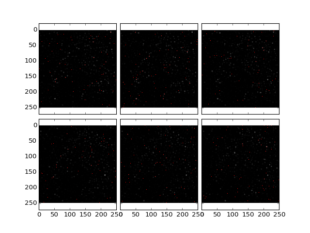
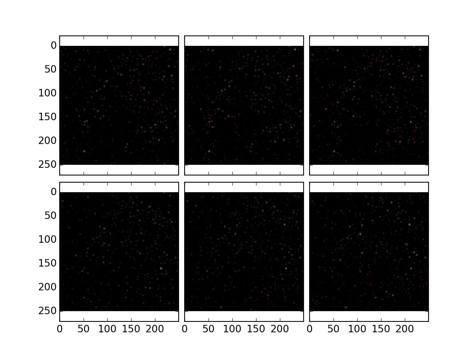
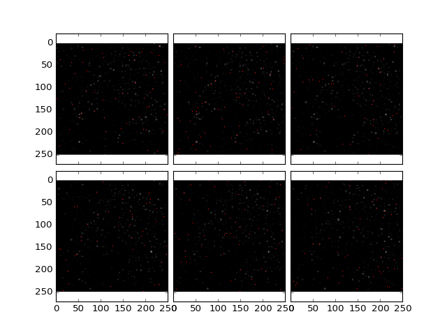
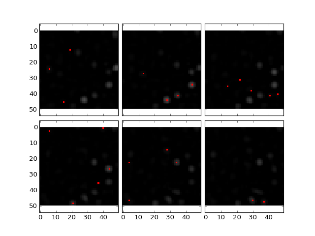
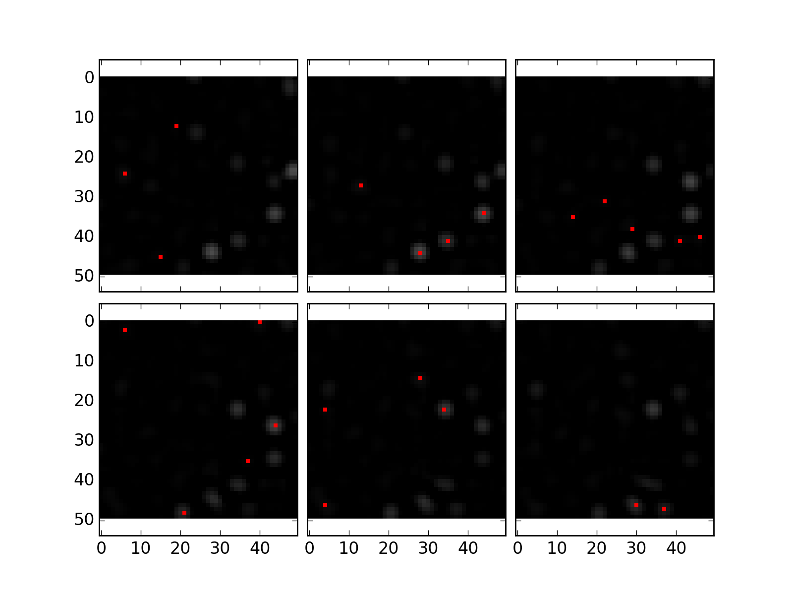
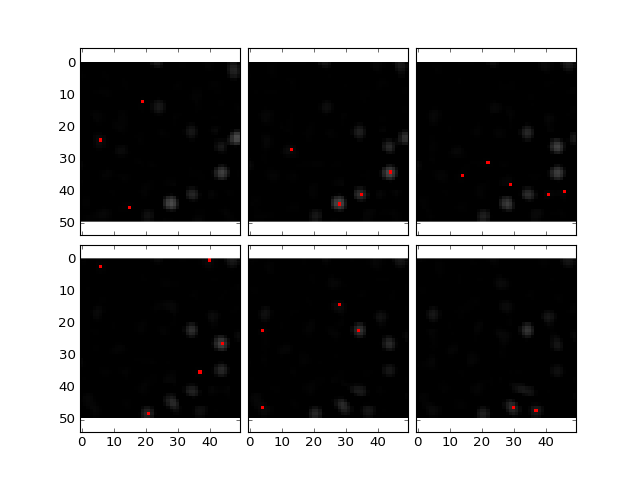
We can also overlay the cell coordinates in an image:

>>> plt.plotOverlayPoints(data, cells, z = (10,16))

(Source code, png, hires.png, pdf)

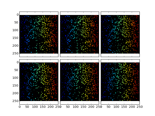
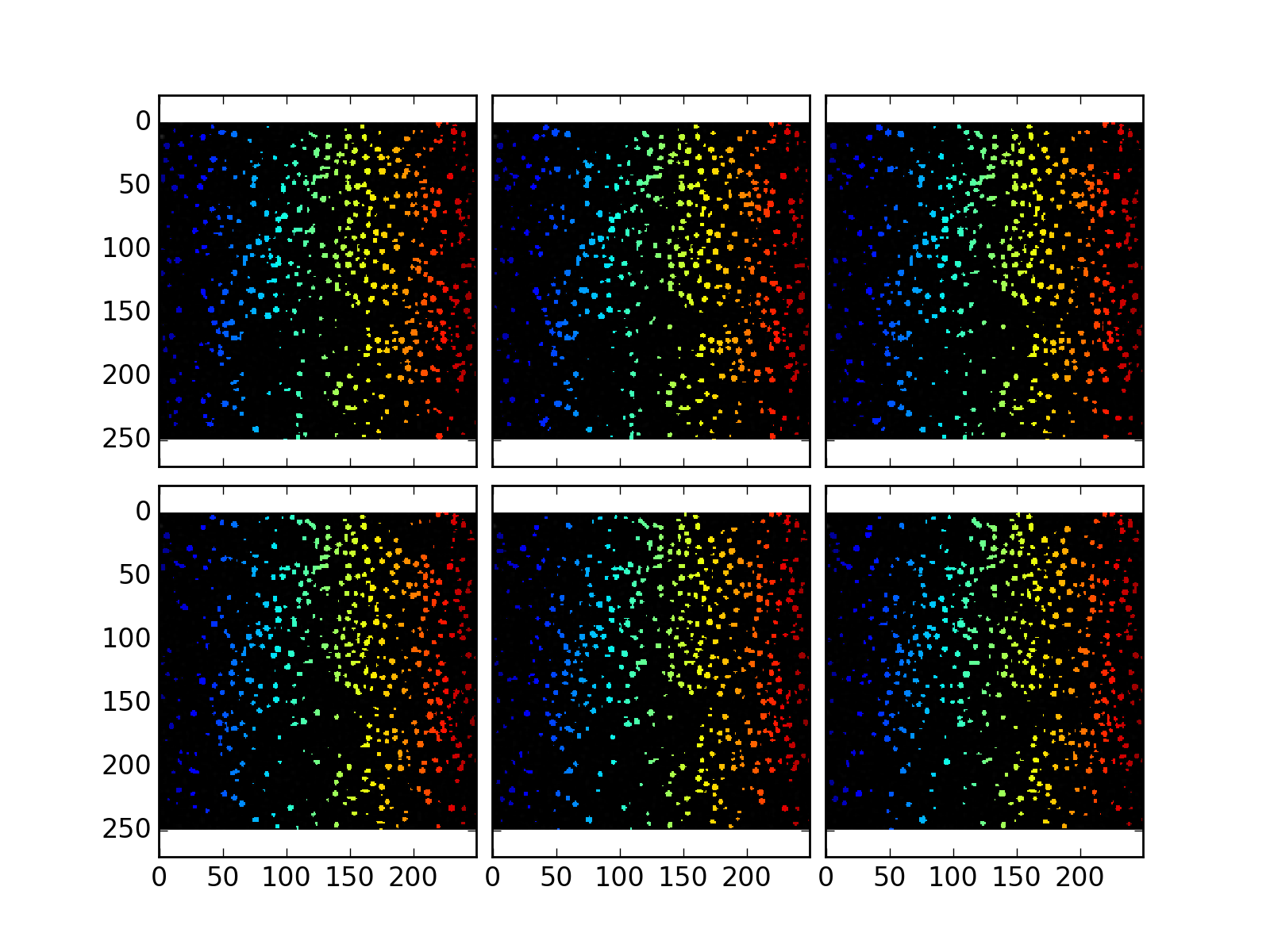
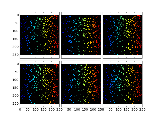
Cell Shape Detection

Finally once the cell centers are detected the ClearMap.ImageProcessing.CellShapedetection module can be used to detect the cell shape via a watershed.

>>> from ClearMap.ImageProcessing.CellSizeDetection import detectCellShape
>>> dataShape = detectCellShape(dataDoG, cells, threshold = 15);
>>> plt.plotOverlayLabel(dataDoG / dataDoG.max(), dataShape, z = (10,16))

(Source code, png, hires.png, pdf)

Now we can perform some measurements:

>>> from ClearMap.ImageProcessing.CellSizeDetection import findCellSize,\
>>>                                                        findCellIntensity
>>> cellSizes = findCellSize(dataShape, maxLabel = cells.shape[0]);
>>> cellIntensities = findCellIntensity(dataBGR, dataShape, maxLabel = cells.shape[0]);

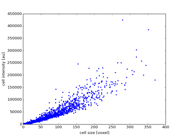
and plot those:

>>> import matplotlib.pyplot as mpl
>>> mpl.figure()
>>> mpl.plot(cellSizes, cellIntensities, '.')
>>> mpl.xlabel('cell size [voxel]')
>>> mpl.ylabel('cell intensity [au]')

(Source code, png, hires.png, pdf)